Hyperspectral satellite imagery for Earth observation

Watch the lightning talk

What is hyperspectral imagery?

Until recently, imaging satellites used cameras that capture the Earth in a few frequency bands. Multispectral sources typically cover the optical red, green, and blue bands of visible light in addition to a few other frequency ranges.

But a revolution is underway. A growing number of satellites equipped with hyperspectral cameras are going to allow us to observe the Earth in extraordinary detail across a large frequency range — well beyond what the human eye can see, and in much more detail than existing multispectral sensors such as Landsat or Sentinel-2.

Hyperspectral imagery enables applications such as tree and plant species identification, monitoring of air quality (particulate and gaseous) and water quality (e.g. algal bloom detection), tree health observation, and more.

Compare visible light to multi- and hyperspectral images

Imaging Type & Example use case

Visible light

3 spectral bands

A RGB image can be used to identify vegetation by shape and color

Multispectral

5-35 spectral bands

A 13-band Sentinel-2 image can be used to differentiate between some crops and detect plants under stress.

Hyperspectral

100s of spectral bands

The 224-band AVIRIS sensor enables detection of plant chemical composition and physiology changes attributed to weeds, diseases, or nutrient deficiency.

Satellite image & spectral bands

Move your mouse over the image

360nmWavelength in nm2500nm

The visualization above shows one spectral band at a time. The amount of data contained in a single image can also be represented as a hyperspectral cube.

Hyperspectral data cube

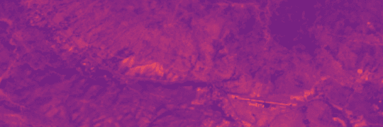
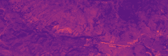
Different materials can often be identified by their characteristic spectral signature. Hyperspectral imaging sensors cover a larger frequency spectrum in narrow, continuous frequency bands. They enable the capture and identification of spectral profiles, such as of healthy (green-stage) and stressed (red-stage) conifers in California.

Explore the spectral profiles in an hyperspectral image

Move your mouse over the image to see the spectral profile in each pixel

AVIRIS images contain 224 datapoints in each pixel. We can compare them with reference spectral profiles known from material science. And tracking changes over time enables measurement of tree health, etc.

Selected pixel

Manually comparing spectral profiles is inefficient at scale. Using machine learning we can train a model to identify the spectral characteristics of different materials. New imagery can then be classified more quickly and at scale.

Techniques for production of actual analyses are still in an early stage. Hyperspectral imagery is currently limited and ground truth and model training data is scarce.

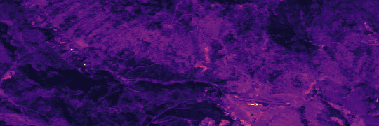
The image below shows early results from our tree health study area in California. Here, we used hyperspectral imagery to distinguish between healthy (green-stage) conifers and conifers under stress (red-stage). These results are from an ML model that works on 224-band AVIRIS imagery.

See how a machine learning model can detect conifer health

Move your mouse over the image

Hyperspectral imageWhat the human eye can see

Element 84 R&D vegetation modelUsing machine learning on spectral profiles

These are early results shown for illustration only.

Red-stage probability

Green-stage probability

Other

Hyperspectral at Element 84

NASA expects to see a major increase in the number of hyperspectral data sets in the coming years. Supported by an innovation research grant from NASA, Element 84 created a reusable, open source data processing pipeline for serving and analyzing hyperspectral imagery.

Our pipeline for hyperspectral imagery processing on the web

Image preparation

We retrieve required scenes, re-encode them to formats suitable for cloud processing such as Cloud Optimized GeoTIFF, and place them in cloud storage using Amazon Web Services (AWS).

Hyperspectral STAC catalog

We catalog imagery using the SpatioTemporal Asset Catalog (STAC) specification for serving geospatial datasets on the web. We use an open-source Franklin server to index imagery and serve features. Franklin lets us query and filter imagery collections by place, time, and spectral coverage.

Image processing & machine learning

We use the Raster Vision geospatial machine learning library to process images using Kubernetes/Argo and AWS.

Interactive, user-friendly web apps

We use a research-driven user experience design process to create actionable and easy-to-use web applications using React.

Work with us on your hyperspectral project

Element 84 is a woman-owned small business that works with public, private, and non-profit sector clients to develop geospatial data processing pipelines and build software.

Get in touch at element84.com/who-we-are/contact-us/